What is a Confusion Matrix in Machine Learning?

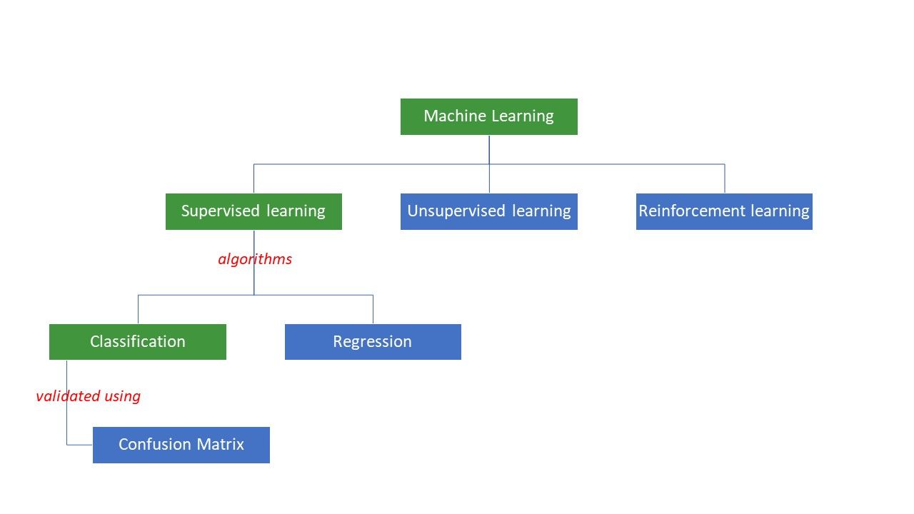
A confusion matrix is a metric to evaluate the performance of the classification type of supervised machine learning algorithms.

What is a Confusion Matrix?

We, humans, perceive things differently – even truth and lies. What may seem a 10cm long line to me may seem like a 9cm line to you. But the actual value may be 9, 10, or something else. What we guess is the predicted value!

Just like our brain applies our own logic to predict something, machines apply various algorithms (called machine learning algorithms) to arrive at a predicted value for a question. Again, these values might be the same or different from the actual value.

In a competitive world, we would like to know whether our prediction is right or not to understand our performance. Same way, we can determine a machine learning algorithm’s performance by how many predictions it made correctly.

So, what’s a machine learning algorithm?

Machines try to arrive at certain answers to a problem by applying certain logic or set of instructions, called machine learning algorithms. Machine learning algorithms are of three types – supervised, unsupervised, or reinforcement.

The simplest types of algorithms are supervised, where we already know the answer, and we train the machines to arrive at that answer by training the algorithm with a lot of data – the same as how a child would differentiate between people of different age groups by looking at their features over and again.

Supervised ML algorithms are of two types – classification and regression.

Classification algorithms classify or sort data based on some set of criteria. For example, if you want your algorithm to group customers based on their food preferences – those who like pizza and those who do not like pizza, you’d use a classification algorithm like decision tree, random forest, naïve Bayes, or SVM (Support Vector Machine).

Which one of these algorithms would do the best job? Why should you choose one algorithm over the other?

Enter confusion matrix….

A confusion matrix is a matrix or table that gives information about how accurate a classification algorithm is in classifying a dataset. Well, the name is not to confuse humans, but too many incorrect predictions probably mean that the algorithm was confused😉!

So, a confusion matrix is a method of evaluating the performance of a classification algorithm.

How?

Let’s say you applied different algorithms to our previously mentioned binary problem: classify (segregate) people based on whether they like or do not like pizza. To evaluate the algorithm that has values closest to the correct answer, you would use a confusion matrix. For a binary classification problem (like/dislike, true/false, 1/0), the confusion matrix gives four grid values, namely:

• True Positive (TP)
• True Negative (TN)
• False Positive (FP)
• False Negative (FN)

What are the four grids in a confusion matrix?

The four values determined using the confusion matrix form the grids of the matrix.

True Positive (TP) and True Negative (TN) are the values correctly predicted by the classification algorithm,

• TP represents those who like pizza, and the model classified them correctly,
• TN represents those who do not like pizza, and the model classified them correctly,

False Positive (FP) and False Negative (FN) are the values that are wrongly predicted by the classifier,

• FP represents those who don’t like pizza (negative), but the classifier predicted that they like pizza (wrongly positive). FP is also called a Type I error.
• FN represents those who like pizza (positive), but the classifier predicted they don’t (wrongly negative). FN is also called Type II error.

To further understand the concept, let’s take a real-life scenario.

Let’s say you have a dataset of 400 people that underwent the Covid test. Now, you got the results of various algorithms that determined the number of Covid positive and Covid negative people.

Here are the two confusion matrices for comparison:

By looking at both, you might be tempted to say that the 1^st algorithm is more accurate. But, to get a concrete result, we need some metrics that can measure the accuracy, precision, and many other values that prove which algorithm is better.

Metrics using confusion matrix and their significance

The main metrics that help us decide whether the classifier made the right predictions are:

#1. Recall/Sensitivity

Recall or Sensitivity or True Positive Rate (TPR) or Probability of Detection is the ratio of the correct positive predictions (TP) to the total positives (i.e., TP and FN).

R = TP/(TP FN)

Recall is the measure of correct positive results returned out of the number of correct positive results that could have been produced. A higher value of Recall means there are fewer false negatives, which is good for the algorithm. Use Recall when knowing the false negatives is important. For example, if a person has multiple blockages in the heart and the model shows he is absolutely fine, it could prove to be fatal.

#2. Precision

Precision is the measure of the correct positive results out of all the positive results predicted, including both true and false positives.

Pr = TP/(TP FP)

Precision is quite important when the false positives are too important to be ignored. For example, if a person does not have diabetes, but the model shows so, and the doctor prescribes certain medicines. This can lead to severe side effects.

#3. Specificity

Specificity or True Negative Rate (TNR) is correct negative results found out of all the results that could have been negative.

S = TN/(TN FP)

It is a measure of how well your classifier is identifying the negative values.

#4. Accuracy

Accuracy is the number of correct predictions out of the total number of predictions. So, if you found 20 positive and 10 negative values correctly from a sample of 50, the accuracy of your model will be 30/50.

Accuracy A = (TP TN)/(TP TN FP FN)

#5. Prevalence

Prevalence is the measure of the number of positive results obtained out of all the results.

P = (TP FN)/(TP TN FP FN)

#6. F Score

Sometimes, it is difficult to compare two classifiers (models) using just Precision and Recall, which are just arithmetic means of a combination of the four grids. In such cases, we can use the F Score or F1 Score, which is the harmonic mean – which is more accurate because it doesn’t vary too much for extremely high values. Higher F Score (max 1) indicates a better model.

F Score = 2*Precision*Recall/ (Recall Precision)

When it is vital to take care of both False Positives and False Negatives, the F1 score is a good metric. For example, those who are not covid positive (but the algorithm showed so) need not be unnecessarily isolated. Same way, those that are Covid positive (but the algorithm said they are not) need to be isolated.

#7. ROC curves

Parameters like Accuracy and Precision are good metrics if the data is balanced. For an imbalanced dataset, a high accuracy may not necessarily mean the classifier is efficient. For example, 90 out of 100 students in a batch know Spanish. Now, even if your algorithm says that all 100 know Spanish, its accuracy will be 90%, which may give a wrong picture about the model. In cases of imbalanced datasets, metrics like ROC are more effective determiners.

ROC (Receiver Operating Characteristic) curve visually displays the performance of a binary classification model at various classification thresholds. It is a plot of TPR (True Positive Rate) against FPR (False Positive Rate), which is calculated as (1-Specificity) at different threshold values. The value that’s closest to 45 degrees (top-left) in the plot is the most accurate threshold value. If the threshold is too high, we will not have many false positives, but we will get more false negatives and vice versa.

Generally, when the ROC curve for various models is plotted, the one that has the largest Area Under the Curve (AUC) is considered the better model.

Let us calculate all the metric values for our Classifier I and Classifier II confusion matrices:

We see that precision is more in classifier II whereas accuracy is slightly higher in classifier I. Based on the problem at hand, decision-makers can select Classifiers I or II.

N x N confusion matrix

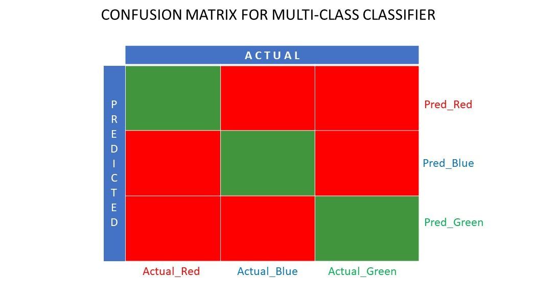
So far, we have seen a confusion matrix for binary classifiers. What if there were more categories than just yes/no or like/dislike. For example, if your algorithm was to sort images of red, green, and blue colors. This type of classification is called multi-class classification. The number of output variables decides the size of the matrix too. So, in this case, the confusion matrix will be 3×3.

Summary

A confusion matrix is a great evaluation system as it gives detailed information about the performance of a classification algorithm. It works well for binary as well as multi-class classifiers, where there are more than 2 parameters to be taken care of. It is easy to visualize a confusion matrix, and we can generate all the other metrics of performance like F Score, precision, ROC, and accuracy using the confusion matrix.

You may also look at how to choose ML algorithms for regression problems.